A production guide to compaction strategies, parameter tuning, maintenance sequencing, and monitoring — covering the control-plane approach that automates these operations, and the manual Spark path for full DIY control.

If you run Iceberg in production, your tables are degrading right now. Not because you configured something wrong — because that's what Iceberg tables do under continuous writes. Streaming jobs create thousands of tiny files. CDC pipelines pile up delete files. Manifest lists grow until planning takes longer than the query. And nobody notices until a dashboard times out or a cost report spikes.

Compaction is the fix. It merges small files into larger ones, sorts data so queries skip irrelevant files, resolves accumulated deletes, and cleans up metadata. It is the single highest-leverage maintenance operation you can run. A well-compacted table routinely queries 10× faster, stores 50% less junk, and costs a fraction of what it cost the day before. A neglected table silently gets worse every hour.

This guide covers everything: how Iceberg stores data (and why that design causes degradation), the three compaction strategies, every parameter that matters, file group mechanics, streaming conflict avoidance, the full four-step maintenance pipeline, snapshot retention, manifest rewriting, health monitoring, sort column selection, and layout simulations.

It also covers two fundamentally different operational models — a lakehouse control plane that handles compaction autonomously, and manual Spark procedures with Airflow DAGs for teams that prefer full control. Both work. They scale differently, and this guide explains why.

1. How Iceberg Stores Data

To understand compaction, you need to understand what you're compacting. An Iceberg table is not a directory of Parquet files. It is a metadata tree with four layers, each serving a specific role in query planning:

Catalog
  └── metadata.json          ← current table state, schema, partition spec
        └── Snapshot          ← immutable point-in-time version
              └── Manifest List (.avro)  ← references all manifest files
                    └── Manifest Files (.avro)  ← per-file statistics
                          └── Data Files (.parquet)  ← actual rows

Every write operation — INSERT, MERGE INTO, DELETE, UPDATE — creates a new snapshot. The snapshot points to a manifest list, which references one or more manifest files. Each manifest file records metadata about the data files it tracks: partition values, column-level min/max bounds, row count, file size, null counts. The data files themselves are Parquet files on S3, GCS, or ADLS.

This structure is what gives Iceberg its power. Atomic commits. Time travel. Schema evolution. Hidden partitioning. Concurrent reads and writes. But every one of those features comes with a metadata cost. Every micro-batch commit adds a snapshot. Every snapshot adds manifest entries. Every tiny file adds another entry for the query planner to evaluate. The metadata tree grows continuously, and the engine must walk it before reading a single row of actual data.

How data skipping works (and why sort order matters)

When a query hits an Iceberg table, the engine doesn't scan every file. It prunes at three levels:

Level 1 — Manifest list pruning. The manifest list contains partition summaries for each manifest. If a query filters on event_date = '2026-09-01' and a manifest's partition summary shows it only covers June, the engine skips the entire manifest without opening it.

Level 2 — Manifest file pruning. For each surviving manifest, the engine evaluates per-file column statistics. A data file with customer_id min=10000, max=19999 gets skipped when the query filters for customer_id = 42. This is where sort order changes the game: if a file's rows are sorted by customer_id, the min/max range is tight — maybe covering only 10,000 IDs. If the rows are unsorted, the min is 1 and the max is 10,000,000, and the file can never be pruned on that column.

Level 3 — Parquet row group pruning. Inside each data file, Parquet organizes rows into row groups (typically 128 MB each). Each row group carries its own min/max column statistics in the Parquet footer. On a sorted file, row groups cover narrow value ranges and most get skipped. On an unsorted file, every row group's range spans the full column domain, and nothing gets skipped.

This three-level pruning is why sort compaction delivers 10× query speedups and bin-pack alone often doesn't change query latency at all. Bin-pack fixes the file count problem. Sort fixes the data skipping problem. They are complementary, not interchangeable.

For a detailed walkthrough of each pruning level, see Apache Iceberg Query Planning Explained.

2. How Tables Degrade

Table degradation is not one problem — it is four, and they compound.

Small files

Streaming ingest is the primary cause. A Flink job committing every 30 seconds produces 2,880 commits per day. If each commit writes to 4 partitions, that's 11,520 new files per day, most between 1 and 50 MB. After a month without compaction, the table has 345,600 files. Every query must evaluate every file's metadata during planning, and every surviving file requires a separate S3 GET request, a Parquet footer parse, and reader initialization overhead.

The numbers get concrete fast. On S3, each GET request costs $0.0004 and takes 5–50 ms of latency. A query hitting 10,000 small files pays $4 in S3 API costs and spends 50–500 seconds just on request overhead before reading a single byte of data. The same data in 100 files of 300 MB each costs $0.04 and finishes in under a second.

A 500 GB table with 100,000 files averaging 5 MB typically plans a query in 15–30 seconds. The same table compacted to 2,000 files at 256 MB plans in under 1 second. That's not a benchmark number — it's the difference between a usable dashboard and one that times out.

Merge-on-read delete accumulation

Iceberg V2/V3 handles DELETE and UPDATE operations with merge-on-read: instead of rewriting the base data file, the engine writes a small delete file listing which rows are removed. This is fast for the writer but expensive for every reader. Each query must load every delete file, build a skip set, and reconcile it against the base data during the scan.

A CDC pipeline processing 10,000 updates per hour creates delete files on every commit. After a week without compaction, a single partition may have hundreds of delete files. A query that would normally take 2 seconds now takes 30, because the engine spends most of its time doing the merge-on-read reconciliation.

V2 position deletes store (file_path, row_position) pairs as Parquet files. The reader must perform an O(n) merge join against each base data file. V3 deletion vectors replace this with Roaring Bitmaps in Puffin files — a single compact bitmap per data file, enabling O(1) lookups. AWS benchmarks show V3 deletion vectors deliver 55% faster delete operations, 23–28% faster reads, and 73% less metadata storage compared to V2. But even with V3, periodic compaction is still needed to physically remove deleted rows and reclaim storage.

Manifest proliferation

Each commit creates new manifest entries. A streaming table producing 2,880 commits per day accumulates manifests fast. With 43,200 manifest entries after two weeks, the query planner must parse hundreds of megabytes of Avro metadata before identifying which data files to read. Teams have seen planning time drop from 45 seconds to under 2 seconds after a single manifest rewrite — the query execution itself was never slow; the planning was.

Snapshot bloat

Without expiration, snapshots accumulate indefinitely. A streaming table creating 3.2 snapshots per hour accumulates 2,300 per month. Each snapshot keeps its referenced files alive on storage, preventing garbage collection. The metadata file grows, and operations like time travel queries must traverse a longer snapshot chain.

These four problems compound. More small files means more manifest entries. More manifests means slower planning. Slower planning means more engine CPU. More engine CPU means higher cost. And through all of this, the table looks fine from the outside — queries still return correct results, they just take 10× longer and cost 10× more.

3. Two Paths: Manual Operations vs. a Control Plane

There are two fundamentally different ways to solve this. Both work. They scale differently, and the choice depends on where you are today and where you're going.

Path A: Lakehouse control plane

A data warehouse handles compaction for you — that's part of the managed deal. An open lakehouse doesn't, because the architecture is deliberately decoupled: you own the data in open formats, any engine can read it, but nobody owns the maintenance.

A lakehouse control plane fills that gap. It's the operational intelligence layer between your catalogs and query engines — it monitors every table, decides what maintenance each one needs, runs it in the right sequence, and learns from the results.

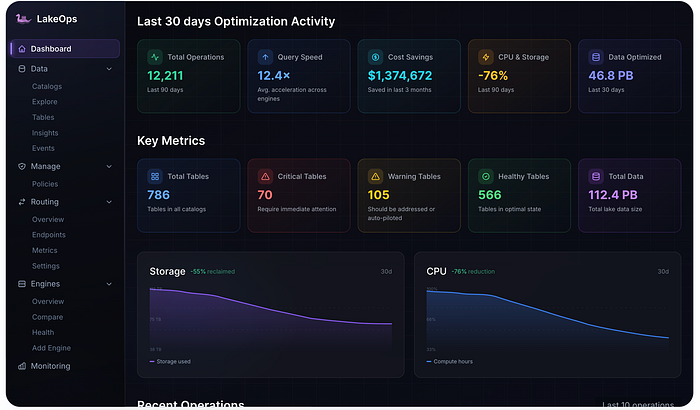
LakeOps is the control plane built for Apache Iceberg. It connects to your existing catalogs (AWS Glue, REST/Polaris, S3 Tables, Nessie, Gravitino) and engines (Trino, Spark, Snowflake, Athena, DuckDB, Flink) without moving data or changing pipelines, and operates in a continuous closed loop:

1. Sense — collects structural signals from every table: file count, average file size, small-file ratio, delete-file accumulation, manifest depth, snapshot age, write velocity. Simultaneously collects query telemetry from every connected engine: which columns appear in WHERE, JOIN, and GROUP BY clauses, how frequently, from which engine.

2. Plan — scores each table as Healthy, Warning, or Critical. Determines which operations to run, in what order, with what parameters. Selects the optimal compaction strategy and sort order based on combined telemetry. Identifies partitions with active writers and excludes them.

3. Optimize — executes the sequenced maintenance pipeline (expire → orphans → compact → manifests) on a purpose-built Rust engine. Not Spark — a dedicated read-merge-write engine built on Apache DataFusion with bounded memory, no JVM, no GC pauses, and no OOM.

4. Learn — measures outcomes (files before/after, planning latency change, query speed improvement, bytes reclaimed) and feeds results back. Sort orders adapt when query patterns shift. Cadence tunes itself to write velocity. Each cycle gets better.

You choose how much control to keep. LakeOps supports three modes: Autopilot (everything runs autonomously — most teams land here after initial confidence), Manual Approval (the system recommends operations and you approve before execution — good for onboarding), and Policy-driven (you define declarative policies for compaction thresholds, retention windows, sort strategies, and cleanup schedules — they enforce themselves across every catalog and table, and new tables inherit them automatically).

Setup takes about 10 minutes. You register your catalogs and engines — LakeOps connects through standard catalog APIs. Only metadata is processed; data never leaves your storage, is never copied, never retained.

Compaction itself runs on a purpose-built Rust engine based on Apache DataFusion — zero-copy Arrow columnar pipeline, bounded memory with disk spill, lock-free parallelism. No JVM, no garbage collection, no cluster provisioning, no OOM. On the same 200 GB / 600M-row table and hardware, S3 Tables compaction took 6,300 seconds (~32 MB/s), Spark took 1,612 seconds (~350 MB/s, high OOM risk, ~$50/TB), and LakeOps finished in 221 seconds (2,522 MB/s, zero OOM risk, ~$5/TB). Production tables at TB scale show the same pattern — a 1.2 TB table compacted from 11,957 to 3,270 files in 11 minutes. Full benchmarks on compaction page.

The result: streaming tables compact hourly, batch tables daily, healthy tables get skipped — no wasted compute. The most degraded tables run first. No cron schedules, no per-table DAGs, no manual sort order selection. For a deep dive on what a control plane is and why open lakehouses need one, see What Is a Data Lakehouse Control Plane?

Path B: Manual — Spark, Airflow, and scripts

Iceberg ships compaction as a Spark SQL stored procedure: rewrite_data_files. You call it with a strategy, parameters, and a WHERE clause to avoid conflicting with active writers. You build an Airflow DAG to schedule the four maintenance operations in the correct sequence. You write SQL against Iceberg metadata tables to check when compaction is needed. You tune Spark executor memory and file group sizes to avoid OOM.

This path gives you full control and no vendor dependency. For a team managing 10–50 tables with batch workloads, it works well. The rest of this guide covers every manual detail so you can do it right — and also shows what the control plane handles automatically at each step.

Where manual breaks down: per-table DAGs become a maintenance burden. Sort orders go stale when query patterns change. OOM and conflict handling require on-call intervention. At 200+ tables, the scripts themselves need a team.

The rest of this guide covers compaction in full depth. Where the two approaches differ in practice, both paths are shown.

4. Compaction Strategies

Iceberg's rewrite_data_files supports three strategies. Each solves a different problem, and choosing wrong means paying the compute cost of compaction while getting zero benefit.

Bin-pack

Bin-pack reads small files and packs them into target-sized files without sorting. It solves the file count problem: fewer files means fewer S3 GET requests, less manifest overhead, faster planning. It does not improve data skipping — min/max statistics stay the same, just packed into larger files.

Bin-pack is the cheapest strategy. It reads each file once, writes output files at the target size, and commits. Minimal CPU, minimal memory, fast execution. It is the right choice when:

• The table serves full-partition scans (daily aggregations, ETL) where predicate pushdown doesn't matter
• You need immediate file count reduction on a streaming table and can run sort later
• The table is small enough that the difference between sorted and unsorted is negligible (under ~50 GB)

The limitation: after bin-pack, a query filtering on customer_id = 42 still opens every file, because no file's min/max range is tight enough to prove it doesn't contain customer 42. On a 500 GB table, that can mean scanning all 500 GB instead of 50 GB.

Sort

Sort compaction reads files, sorts all rows by one or more columns, and writes new files. The sort makes Parquet row group statistics tight: after sorting by event_date, each file covers a narrow date range. A query filtering on event_date BETWEEN '2026-09-01' AND '2026-09-07' reads 7 files instead of 2,000.

Sort is the strategy that delivers the 10× query speedup. But it only works when the sort columns match the query predicates. If you sort by event_date and the query filters on customer_id, the sort did nothing. Choosing the right sort columns is the single most important decision in compaction — more on that in section 12.

Sort is more expensive than bin-pack: it must hold sort state in memory, and it produces write amplification (every file in the group gets rewritten, even if its content would have been fine). On a 500 GB table, the difference between a good sort order and a bad one can be the difference between 52 seconds and under 6 for a typical analytical query.

Z-order

Z-order (Morton curve) applies a space-filling curve to interleave bits from 2–4 sort columns, clustering data across multiple dimensions simultaneously. Linear sort optimizes hard for the first column and weakly for subsequent ones. Z-order distributes the benefit evenly across all specified columns.

The trade-off: Z-order is the most expensive strategy (CPU-intensive bit interleaving), and the per-column pruning is less aggressive than linear sort. A query filtering only on the primary sort column will skip fewer files with Z-order than with linear sort.

Z-order is the right choice when:

• Queries filter on different column combinations unpredictably — one analyst filters by campaign_id, another by region, a dashboard by event_date
• The table is large enough (100+ GB) to justify the compute cost
• You can limit to 2–4 high-cardinality columns — beyond 4, the locality guarantee weakens and the overhead grows without proportional benefit

Hilbert curves are an emerging alternative that avoids Z-order's quadrant-boundary discontinuities. Early benchmarks show ~57% file skip rate versus Z-order's ~46% on the same dataset. Not yet in mainline Iceberg, but available through LakeOps's Rust engine.

On the manual path, you choose the strategy per table and maintain that choice as workloads evolve. When an append-only table starts receiving deletes, or an ad-hoc table develops a dominant filter column, someone needs to notice and switch the strategy.

On the control plane path, LakeOps selects the strategy per table based on write velocity, query patterns, and delete-file accumulation — and re-evaluates on every cycle. A table that was bin-pack-only because it had no dominant filter pattern gets upgraded to sort when cross-engine telemetry reveals that 80% of queries now filter on event_date. You can override via policy (e.g., "always sort this table by customer_id, event_date") or let the system decide. For a deeper comparison, see Iceberg Compaction Strategies: A Practical Guide.

5. The rewrite_data_files Procedure

This is the Spark SQL entry point for compaction:

CALL catalog.system.rewrite_data_files(
  table => 'db.events',
  strategy => 'sort',
  sort_order => 'event_date ASC, customer_id ASC',
  options => map(
    'target-file-size-bytes',       '536870912',
    'min-file-size-bytes',          '402653184',
    'max-file-size-bytes',          '966367641',
    'min-input-files',              '5',
    'partial-progress.enabled',     'true',
    'partial-progress.max-commits', '10',
    'max-file-group-size-bytes',    '5368709120',
    'max-concurrent-file-group-rewrites', '3',
    'use-starting-sequence-number', 'true'
  )
)

Most teams run with defaults and then wonder why compaction is slow, crashes, or causes conflicts. On the control plane path, these parameters are auto-tuned per table — but understanding what each one does matters regardless of which path you take. Here is every parameter and why the default is often wrong for production.

target-file-size-bytes

Controls the output file size. Iceberg applies a tolerance window: files between 75% and 180% of the target are left alone. Files below 75% are candidates for merging. Files above 180% may be split.

The right target depends on the workload:

• 128 MB — Point lookups, feature stores. Smaller files mean finer-grained pruning when the query selects individual records.
• 256 MB — Mixed workloads. The most common default for production tables under 1 TB. Good balance between pruning granularity and S3 overhead.
• 512 MB — Full-scan analytics on large tables (1+ TB). Fewer files means less planning overhead and fewer S3 requests. Default in Iceberg.

One subtle interaction: target file size and partition cardinality. If your table is partitioned by event_date and each day has 500 MB of data, a 512 MB target produces one file per partition — which means zero parallelism for queries scanning a single day. A 128 MB target produces four files per partition, enabling four-way parallel reads. Match the target to the per-partition data volume, not just the total table size.

partial-progress.enabled

This is the single most important production setting. Default is false. Set it to true.

Without partial progress, Iceberg groups all files into file groups, rewrites them, and commits everything as a single atomic operation. If any file group conflicts with a concurrent writer (which is inevitable on streaming tables), the entire compaction job is rolled back. A 4-hour compaction run that fails on file group 8 of 10 means 4 hours of compute wasted and a still-fragmented table.

With partial-progress.enabled = true, Iceberg commits each file group independently. If group 8 conflicts, groups 1–7 and 9–10 stay committed. Set max-commits to 10–20 to control the commit granularity.

use-starting-sequence-number

Set to true for streaming tables. This tells compaction to only rewrite files that existed at the start of the compaction run, ignoring files written by concurrent streaming jobs during compaction. It reduces conflict potential significantly.

min-input-files

Default is 5. This prevents wasteful compaction: if a file group has fewer than 5 files, it's skipped. On tables with low write frequency, lowering this to 2–3 can help catch partitions with just a few undersized files. On high-frequency tables, the default is fine.

Delete file thresholds

For merge-on-read tables (V2/V3 with position or equality deletes), two parameters control when delete-heavy files get pulled into compaction:

• delete-file-threshold (default: disabled) — if a data file has more than this many associated delete files, it becomes a compaction candidate regardless of its size. Set to 1–5 for CDC-heavy tables.
• delete-ratio-threshold (default: disabled) — triggers compaction when the ratio of deleted rows to total rows exceeds this value. Set to 0.1 for tables with high update rates.

Without these settings, a perfectly-sized 256 MB file with 500 associated delete files will never be compacted — and every query will pay the merge-on-read tax on it.

That's 9 parameters per table, each with interactions that depend on table size, write velocity, delete patterns, partition cardinality, and query workload. On the manual path, you own every one of them. On the control plane path, LakeOps auto-tunes these per table based on observed health signals — including adjusting delete thresholds when mutation rate changes, tightening file group sizes before a table hits Spark OOM territory, and enabling partial progress by default. You can override any parameter via policy if you need specific behavior.

6. File Groups, Parallelism, and Spark OOM

This is where most production compaction jobs die. Understanding file groups is essential for survival.

Iceberg divides compaction work into file groups — bundles of files up to max-file-group-size-bytes (default: 100 GB). Each group is rewritten independently, allowing parallelism controlled by max-concurrent-file-group-rewrites (default: 5). The problem: with 5 concurrent rewrites of 100 GB groups, Spark can be managing metadata and sort state for 500 GB of data simultaneously.

Sort compaction is particularly memory-hungry. Sorting requires holding sort keys in memory, and with large file groups, the sort state can exhaust JVM heap. The result: OOM.

Production-safe settings:

options => map(
  'max-file-group-size-bytes',          '5368709120',   -- 5 GB
  'max-concurrent-file-group-rewrites', '3',
  'partial-progress.enabled',           'true',
  'partial-progress.max-commits',       '20'
)

Spark-level tuning:

• spark.driver.memory = 16g — the driver handles manifest planning, which exhausts default heap on large tables
• spark.executor.memoryOverhead = 2g+ — the default 10% of executor memory is too small for sort compaction
• Enable AQE (spark.sql.adaptive.enabled = true) — lets Spark adjust partitioning based on actual data sizes

Even with tuning, Spark compaction has a fundamental problem: compaction is a narrow, I/O-bound read-merge-write loop. Running it on a general-purpose distributed JVM engine means paying for cluster startup (2–5 min), garbage collection pauses, idle executor overhead, and OOM risk. A table that needs 11 minutes of actual compaction work costs 20+ minutes of wall clock and requires a dedicated cluster.

This is where the control plane path diverges most sharply. LakeOps runs compaction on a purpose-built Rust engine built on Apache DataFusion — zero-copy Arrow columnar pipeline, bounded memory with disk spill, lock-free parallelism. No JVM, no GC, no cluster provisioning. A 1.2 TB table that OOM'd Spark three times finished in 11 minutes on its first try. Production benchmarks on 200 GB / 600M rows, same hardware: S3 Tables compaction took 6,300 seconds (~32 MB/s), Spark took 1,612 seconds (~350 MB/s), LakeOps took 221 seconds (2,522 MB/s). That's 95% faster and roughly 90% cheaper per TB ($5/TB versus $50/TB). And the engine learns: consecutive passes on the same table improve throughput without configuration changes (22 min → 11 min, 925 → 1,572 MB/s on balance_snapshots).

7. Compaction on Streaming Tables

Streaming ingest is the most common source of small files and the hardest environment to compact safely. The core challenge is optimistic concurrency control (OCC).

Iceberg uses OCC for all writes. Each writer reads the current table state, does its work, and attempts to commit. At commit time, Iceberg validates that none of the files the writer modified were also modified by another concurrent writer since the read. If they were, the commit fails with a ValidationException.

The classic scenario: a Flink job is appending to event_date = '2026-09-06' every 30 seconds. A compaction job starts, reads all files in that partition, spends 5 minutes rewriting them, and tries to commit. During those 5 minutes, the Flink job committed 10 new files to the same partition. The compaction commit fails because it's trying to replace files that no longer represent the current state. Without partial progress, the entire compaction run — including work on 50 other partitions that had no conflicts — gets rolled back.

The solution: partition-aware compaction

Never compact the partition that is actively being written to. This eliminates OCC conflicts entirely.

CALL catalog.system.rewrite_data_files(
  table => 'db.clickstream',
  strategy => 'binpack',
  where => 'event_date < current_date() - INTERVAL 1 DAY',
  options => map(
    'partial-progress.enabled',     'true',
    'partial-progress.max-commits', '10',
    'target-file-size-bytes',       '268435456',
    'use-starting-sequence-number', 'true'
  )
)

The WHERE clause restricts compaction to partitions older than today. The streaming writer owns today's partition; compaction owns yesterday and older. When today becomes yesterday, the next compaction cycle picks it up.

This pattern has a subtlety: it assumes writes are neatly partitioned by date. In practice, late-arriving data, backfills, and multi-source ingestion can make "active partitions" less predictable. A Spark ETL backfilling event_date = '2026-06-01' while Flink streams into today means two active partitions, not one.

LakeOps handles this by monitoring actual per-partition commit activity across all connected engines — not just time-based filtering. If a partition received a commit in the last hour from any engine, it's excluded from compaction. When the writer moves on, the next cycle picks it up. This protects against backfills, late arrivals, and multi-engine writes that simple date-based WHERE clauses miss. For a deep dive, see Apache Iceberg Commit Conflicts.

Compaction cadence for streaming tables

If your table receives 14,400 files per day and you compact once at midnight, the table spends 23 hours degraded. Compaction cadence must match write cadence:

• High-frequency streaming (sub-minute commits) — bin-pack every 1–2 hours on cold partitions, sort daily or weekly
• Micro-batch (5–15 minute commits) — bin-pack every 4–8 hours, sort weekly
• Batch (daily loads) — sort after each load completes

On the control plane path, cadence adapts automatically to each table's write velocity. A table committing every 30 seconds gets compacted multiple times per hour. A table that writes once a week gets compacted once. A table nobody writes to gets nothing. No cron schedule can replicate this — it requires observing actual table state. LakeOps also detects when a streaming job completes (e.g., end-of-day ETL finishes) and immediately triggers compaction on the freshly written partitions — closing the gap between write completion and optimal layout. For a complete walkthrough of streaming compaction patterns, see Kafka to Iceberg Compaction — Done Right.

8. Delete File Resolution

Iceberg V2/V3 tables using merge-on-read accumulate two types of delete files, each with different read-time costs.

Position deletes record (file_path, row_position) pairs. At read time, the engine loads each position delete file, sorts it, and performs a merge join against the base data file. With N delete files per data file, the cost is O(N) per file — and N grows with every delete operation. A table with 50 position delete files per data file adds 200–500 ms per file scan.

Equality deletes record column values — "delete every row where order_id = 88213." Useful for streaming writers that know a key but not a physical row position (common in Flink consuming from Kafka). The cost is on the read side: the engine must evaluate every row in every in-scope data file against every equality delete predicate. That's closer to a join than a filter, and it's O(D × R) where D is the number of delete entries and R is the row count.

V3 deletion vectors replace position delete files with Roaring Bitmaps in Puffin files. A single compact bitmap per data file, with O(1) lookups. Multiple deletes to the same file merge into the existing bitmap rather than creating new delete files. This eliminates the N-delete-files-per-data-file scaling problem that made V2 position deletes expensive at scale.

The fix for all three: resolve deletes during compaction. When compaction rewrites files, it reads base data, applies pending deletes (position, equality, and deletion vectors), and writes clean output with zero pending delete overhead. After compaction, queries read clean files with no reconciliation cost.

Key settings for the manual path:

• delete-file-threshold = 1–5 — pull files into compaction when delete files accumulate, even if the data file itself is healthy-sized
• remove-dangling-deletes = true — clean up delete files that reference already-compacted data files

On the control plane path, delete file resolution is automatic and adaptive. LakeOps monitors the delete-to-data ratio per partition continuously. When the ratio crosses a threshold, it triggers compaction that resolves accumulated deletes — producing clean output with zero merge-on-read overhead. The threshold adapts per table: CDC tables with high mutation rates get tighter thresholds (compaction every 1–2 hours on hot partitions), while append-only tables with occasional deletes get looser ones (every 4–8 hours). V3 deletion vectors and equality deletes are both resolved in the same compaction pass. You can set delete thresholds explicitly via policy or let autopilot manage them. For the full mechanics, see Apache Iceberg Delete Files: Reducing Merge-on-Read Overhead.

9. The Maintenance Pipeline

Compaction is one of four interdependent maintenance operations. Running them in the wrong order wastes compute. Running them in the right order compounds their benefit.

1. Expire Snapshots
2. Remove Orphan Files
3. Compact Data Files
4. Rewrite Manifests

Why this order, specifically:

Step 1: Expire snapshots first. Snapshot expiration marks old snapshots as expired and releases the files they exclusively reference. If you compact before expiring, you may rewrite files that expiration would have removed — burning compute on data that's about to be garbage collected. Expire first, compact the survivors.

CALL catalog.system.expire_snapshots(
  table => 'db.events',
  older_than => TIMESTAMP '2026-09-01 00:00:00',
  retain_last => 10,
  stream_results => true
)

Retention tuning matters. Set older_than to at least 2× your longest-running query — a read that opened a snapshot can fail if that snapshot gets expired mid-scan. Set retain_last to at least 2 (never 1 — that leaves zero rollback targets). For streaming tables: 3–7 days, retain_last 25–50. For batch: 7–30 days, retain_last 5–10. For compliance tables with audit requirements, use Iceberg tags on specific checkpoints (end-of-quarter, audit milestones) — tagged snapshots survive expiration automatically. For the full retention framework, see Snapshot Retention and Time Travel.

Step 2: Remove orphan files. Failed writes, aborted jobs, and concurrent operations can leave files on S3 that aren't referenced by any snapshot. These accumulate silently and cost storage. The critical safety rule: use a grace period of at least 72 hours (3 days is the Iceberg default). In-progress writes may have uncommitted files that are valid — cleaning them up corrupts the table.

CALL catalog.system.remove_orphan_files(
  table => 'db.events',
  older_than => TIMESTAMP '2026-09-03 00:00:00'
)

Step 3: Compact data files. Now that expired snapshots and orphans are cleared, compact the surviving files. Every file you compact is genuinely needed — no wasted rewrites on dead data.

Step 4: Rewrite manifests. After compaction changes the file layout, the old manifest organization is stale. Manifest rewriting consolidates fragmented manifests into fewer, larger ones aligned with partition boundaries. This is a metadata-only operation — it doesn't touch data files — and it's cheap. A table with 2,000 tiny manifests (each tracking 10–50 files) can consolidate to 40 manifests (each tracking 500–1,000 files), dropping planning time from 8 seconds to 200 ms.

CALL catalog.system.rewrite_manifests(
  table => 'db.events'
)

Run this after every compaction pass. Teams that master compaction often overlook manifests — a well-compacted table with 2,000 tiny manifests still has slow planning. Manifest rewriting is the cheapest operation with the most outsized benefit. For the full mechanics of manifest optimization at scale, see Iceberg Metadata at Scale.

On the manual path, you build this four-step sequence as an Airflow DAG per table, with each task depending on the previous and error handling at every step. For a walkthrough, see Automating Apache Iceberg Table Maintenance.

On the control plane path, LakeOps runs this exact sequence automatically for every connected table — dependency-ordered, triggered by health signals, with full audit logging. Each step's output is the next step's clean input. Retention windows, orphan cleanup grace periods, and compaction thresholds are configurable via declarative policies — set them once at the namespace or catalog level and every table inherits them, including new tables created after the policy is defined. At 200 tables, that's 200 four-step pipelines running in the correct order without a single DAG to build, debug, or maintain. Every operation is logged with duration, files affected, bytes reclaimed, and the health signal that triggered it — useful for compliance environments that require proof of data lifecycle management.

10. Target File Size: How to Choose

Target file size is table-specific, not universal. The standard guidance of "use 256–512 MB" is correct as a starting point but misses important nuances.

The core trade-off: smaller files enable finer-grained pruning (fewer rows read per query) but create more metadata overhead and more S3 requests. Larger files amortize overhead but reduce parallelism and pruning granularity.

Match the target to the workload:

• Point lookups, feature stores, real-time scoring — 64–128 MB. The query selects a few rows; smaller files mean less data read per hit.
• Mixed analytical workloads — 256 MB. The sweet spot for most tables under 1 TB. Good balance between pruning and S3 efficiency.
• Full-scan analytics, BI dashboards — 256–512 MB. Fewer files means less planning overhead.
• Large tables (10+ TB), petabyte scale — 512 MB. Keeps manifest counts manageable and planning fast.

Match the target to the partition volume. If a daily partition contains 500 MB of data and you set target to 512 MB, you get one file per partition — zero read parallelism for queries scanning a single day. A 128 MB target gives you 4 files per partition, enabling 4-way parallel reads. Check per-partition data volume before setting the target.

On the control plane path, file size is not a static setting — it adapts. LakeOps monitors the file size distribution per table after each compaction pass and evaluates whether the current target is producing the right layout. If a table's files consistently fall below the target shortly after compaction (because of high-frequency appends), the system tightens the trigger threshold or increases compaction frequency. If partition volumes are too small for the configured target (producing single-file partitions with no read parallelism), it adjusts the target down.

You can set file size targets explicitly via policy ("all tables in the analytics namespace target 256 MB"), let autopilot decide based on observed access patterns, or run layout simulations to test candidates before committing. LakeOps's simulation mode tests a proposed file size alongside sort order candidates on an Iceberg branch — so you can see the projected impact on pruning and parallelism before rewriting a single production file. For the full compaction tuning framework, see Optimizing Iceberg Lake Compaction.

11. Monitoring Table Health

Running compaction on a fixed cron schedule is common and consistently wrong. A table receiving 100 writes per hour degrades in 2 hours. A table receiving 1 write per week doesn't need compaction at all. Cron treats them identically.

Health-based monitoring is better. Iceberg exposes everything you need through its system metadata tables:

-- How fragmented are the files?
SELECT
  COUNT(*) AS total_files,
  AVG(file_size_in_bytes) / 1048576 AS avg_mb,
  SUM(CASE WHEN file_size_in_bytes < 67108864 THEN 1 ELSE 0 END) * 100.0
    / COUNT(*) AS small_file_pct
FROM db.events.files
WHERE content = 0;  -- 0 = data files only
-- Which partitions need attention?
SELECT partition, COUNT(*) AS file_count,
       AVG(file_size_in_bytes) / 1048576 AS avg_mb,
       MIN(file_size_in_bytes) / 1048576 AS min_mb
FROM db.events.files
WHERE content = 0
GROUP BY partition
HAVING COUNT(*) > 20 AND AVG(file_size_in_bytes) < 134217728
ORDER BY file_count DESC;
-- How heavy is the metadata?
SELECT
  (SELECT COUNT(*) FROM db.events.manifests) AS manifest_count,
  (SELECT COUNT(*) FROM db.events.snapshots) AS snapshot_count;
-- Delete file burden (V2/V3)
SELECT COUNT(*) AS delete_file_count,
       SUM(record_count) AS pending_deletes
FROM db.events.files
WHERE content IN (1, 2);  -- 1 = position deletes, 2 = equality deletes

Health thresholds:

• Average file size: Healthy = 128–512 MB · Warning = 32–128 MB · Critical = < 32 MB
• Small files (< 64 MB) as percentage: Healthy = < 5% · Warning = 5–20% · Critical = > 20%
• Delete-file-to-data-file ratio: Healthy = < 0.1 · Warning = 0.1–0.5 · Critical = > 0.5
• Manifest count: Healthy = < 100 · Warning = 100–500 · Critical = > 500
• Snapshot count: Healthy = < 1,000 · Warning = 1,000–10,000 · Critical = > 10,000

On the manual path, you build these checks into an Airflow sensor or dbt test, store results somewhere, set up alerting, and trigger the right maintenance operation based on which threshold was breached. For each table. For each metric. With escalation logic and retry handling.

On the control plane path, LakeOps computes these health scores continuously from catalog metadata, for every table, across every catalog. Each table is surfaced as Healthy, Warning, or Critical with a drill-down into which dimensions are degraded (small files, delete accumulation, manifests, snapshots). When a table crosses a threshold, the correct sequenced operation fires automatically. Worst-degraded tables run first — not first-in-first-out. You also get historical health trends: see how a table's file count, average file size, and delete ratio have changed over weeks and months, and whether compaction is keeping up with write velocity or falling behind. That visibility is nearly impossible to get from ad-hoc SQL queries against Iceberg metadata tables.

CONTROL PLANE (PATH A)                   MANUAL (PATH B)
──────────────────────                   ─────────────────
Health scores computed automatically     Write SQL health queries per table
Threshold-driven triggers built in       Build alerting rules + threshold logic
4-step pipeline sequenced per table      Build Airflow DAGs for 4 procedures
Rust engine, no JVM, no tuning           Tune Spark memory, file groups, cron
Active partitions auto-excluded          Debug OCC conflicts at 3 AM
Sort adapts from query telemetry         Quarterly sort-order audits
File size adapts from access patterns    Fixed target, hope it's right
Tables stay healthy automatically        ~2–4 weeks engineering per quarter

12. Choosing Sort Columns

The biggest question in sort compaction — and the one most teams get wrong — is which columns to sort by.

Sort order determines how tight the min/max statistics are in each file and row group. Tight statistics enable data skipping; loose statistics don't. A file sorted by event_date has a min/max range of maybe 1 day — a query filtering on a specific date skips every file whose range doesn't overlap. A file with random row order has a min/max range spanning the entire column domain — nothing gets skipped.

The right sort columns are the ones that appear most frequently in WHERE, JOIN, and GROUP BY clauses across all engines reading the table. Not the columns you think queries use — the columns they actually use.

Manual path: query log analysis

Inspect query history in Trino's query log, Spark's event log, Snowflake's QUERY_HISTORY, Athena's query execution stats. Tally which columns appear in filter and join predicates. If 70%+ of queries filter on the same 1–2 columns, use linear sort. If filters spread across 3–4 columns unpredictably, use Z-order.

The manual approach works at small scale. The problems:

• Each engine stores query history differently — there's no single cross-engine view
• Analysis needs to be repeated quarterly as workloads evolve
• A new dashboard or AI agent can change access patterns overnight
• You're choosing sort columns for hundreds of tables, each with different query patterns

Control plane path: cross-engine telemetry

LakeOps connects to every engine reading your tables and collects telemetry on which columns appear in filter and join predicates — across Trino, Spark, Snowflake, Athena, DuckDB, and Flink simultaneously. It ranks columns by file-pruning impact, applies the optimal sort order during compaction, and adapts when patterns change. A new BI dashboard that filters on region instead of customer_id causes the sort order to adapt on the next compaction pass — no quarterly audit, no manual intervention.

You can override the automatic sort order via policy (e.g., "always sort orders by customer_id, order_date") or let the system decide. In manual approval mode, LakeOps proposes a sort order change and waits for confirmation before applying it — useful during onboarding or for compliance-sensitive tables where layout changes need human sign-off.

Production results: 12× faster queries and 76% less CPU on tables where LakeOps replaced manual sort-order selection. The improvement comes entirely from better data layout — same data, same engines, same queries. For the full architecture, see Apache Iceberg Multi-Engine Architecture.

13. Layout Simulations

Sort compaction on a terabyte table is expensive. If you pick the wrong sort columns, you spend that compute budget for zero improvement. There's no undo — you'd have to re-compact with different columns, doubling the cost.

The safer approach: test layout changes on Iceberg branches before touching production. Iceberg's branching support (since v1.2) lets you create a lightweight metadata copy, apply a candidate sort order, and compare scan statistics — without modifying production data.

LakeOps automates this as layout simulations. You can test multiple strategies simultaneously: sort by event_date, region vs. sort by customer_id, event_date vs. zorder(customer_id, event_date, region). Each strategy runs on its own Iceberg branch, replayed against real production queries from cross-engine telemetry. The results show scan reduction, file count delta, and estimated query speedup side by side. Apply the winner with one action. In autopilot mode, LakeOps runs simulations automatically when it detects query patterns have shifted enough to justify re-evaluating the current sort order — and applies the winner without intervention. In manual approval mode, you see the simulation results and choose when to apply. Production tables stay untouched until you're confident.

Before running sort compaction on any table over 500 GB, simulate the layout change first. If the projected improvement is less than 2×, bin-pack alone may be sufficient — and it's 5–10× cheaper to run.

14. Multi-Engine Compaction

Most production Iceberg deployments serve multiple engines — Spark for ETL, Trino for dashboards, Snowflake for ad-hoc, DuckDB or StarRocks for fast lookups, Flink for streaming.

This creates problems that no single engine can solve:

Sort order conflicts. Trino dashboard queries filter on customer_id. Athena ad-hoc queries filter on event_date. Snowflake exploration filters on region. Which column do you sort by? The answer depends on the combined query mix weighted by frequency and impact — which no single engine sees, because each only logs its own queries.

Compaction ownership. If both Spark and Trino trigger compaction, they conflict with each other. The table needs a single compaction owner with cross-engine visibility. Running compaction on one engine's cluster also means competing with that engine's query workload for resources.

A control plane is the natural single owner. It sits above all engines, sees the combined query telemetry, and runs compaction on its own dedicated engine — no competition with query resources. LakeOps evaluates whether a composite sort, Z-order, or primary/secondary sort best serves the combined workload across all engines. It also prevents compaction conflicts: if Spark ETL and Trino-triggered compaction would both try to rewrite the same table, LakeOps is the single coordinator — no OCC races between competing compaction jobs.

Conclusion

Compaction is the highest-leverage operation you can run on an Iceberg table. The procedure itself is straightforward — rewrite_data_files with the right strategy, the right file size target, and the right partition exclusions. What makes it hard at scale is everything around it: correct sequencing of four interdependent operations, health monitoring across hundreds of tables, cross-engine sort column selection that stays current as workloads evolve, streaming conflict avoidance that handles backfills and late arrivals, and a compaction engine that doesn't cost more than the queries it's supposed to speed up.

The control plane solves all of this structurally and automatically.

LakeOps connects to your existing catalogs and engines, monitors every table's health continuously, runs the full four-step maintenance pipeline in the right order with the right parameters on a Rust engine that costs a fraction of Spark, adapts sort orders from cross-engine telemetry, simulates layout changes before applying them, and handles streaming conflicts through actual commit monitoring — not date-based heuristics. Start in manual approval mode, graduate to autopilot, or define policies and enforce them everywhere. For a hands-on walkthrough, see Iceberg Lakehouse Optimization with LakeOps.

If you're running a small number of tables with batch workloads and prefer full DIY control, the manual path works well. Set partial-progress.enabled = true. Expire snapshots before compacting. Exclude active streaming partitions. Shrink file groups to avoid OOM. Build a solid Airflow DAG for each table. Monitor health thresholds with the SQL queries in section 11. Revisit sort columns quarterly. And when the lake grows past what scripts can sustain — when OOM failures and streaming conflicts generate 3 AM pages, when sort orders go stale because nobody audited them this quarter — the control plane is a natural next step.

Further reading