The architecture, components, and operational reality of building a production open data lakehouse in 2026 — from object storage to autonomous compaction and table management.

The open data lakehouse is the architecture that replaced the data warehouse vs. data lake debate. Instead of choosing between cheap-but-ungoverned storage and expensive-but-transactional compute, you get both — ACID transactions on commodity object storage, with any engine reading and writing through open standards.

But "open data lakehouse" means something specific. It is not a product you purchase from a single vendor. It is a modular architecture assembled from independent, open-source components — each handling one layer of the problem, each swappable without rebuilding the rest. This is what distinguishes it from proprietary lakehouse offerings that bundle everything behind a single vendor's control.

This guide walks through what an open data lakehouse actually is, the components that make it work, where the architecture stands in 2026, and how to operate one in production. If you are evaluating whether to build on open standards or trying to understand what is missing from your current stack, this is the map.

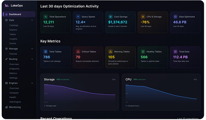
LakeOps is an autonomous control plane purpose-built for the open data lakehouse. It connects to your existing catalogs and engines, then handles the operational layer — compaction, maintenance, observability, governance, and multi-engine routing — that no single open-source component was designed to own. We will reference it throughout where it fills specific gaps in the architecture.

How we got here: warehouse → lake → lakehouse

The open data lakehouse did not appear from nowhere. It evolved from two earlier architectures that each solved half the problem:

Data warehouses gave us structure, governance, and fast SQL. But they stored data in proprietary formats, charged per-compute-cycle pricing, and could not handle unstructured data, streaming, or ML workloads without expensive workarounds. Scaling from terabytes to petabytes meant scaling your invoice proportionally.

Data lakes gave us cheap, infinite-scale storage for any data type. But they provided no transactional guarantees, no schema enforcement, no consistent reads. Without governance, lakes became swamps — landing zones for data that nobody could trust or query reliably.

The lakehouse architecture merges both: warehouse-grade reliability (ACID, schema enforcement, time travel) on lake-grade economics (open formats on object storage). You stop duplicating data between a lake and a warehouse. You stop paying warehouse pricing for storage. You stop sacrificing governance for flexibility.

The open lakehouse goes one step further: every layer uses independent open standards, so no single vendor controls the architecture.

What is an open data lakehouse?

An open data lakehouse combines three ideas:

1. Data lake economics — store everything on cheap object storage (S3, GCS, ADLS). No proprietary formats, no per-byte egress traps, no storage tied to compute.
2. Data warehouse guarantees — ACID transactions, schema enforcement, time travel, consistent reads across concurrent writers. The features that made warehouses reliable, now on open storage.
3. Open, modular components — every layer (format, catalog, compute, operations) is an independent open standard. Swap any piece without rewriting the rest. No single vendor controls the architecture.

The "open" qualifier is load-bearing. Databricks, Snowflake, and Google all offer lakehouse products — but if the table format, catalog, and compute are all proprietary or tightly coupled, you do not have an open lakehouse. You have a vendor platform that uses the word.

An open data lakehouse is only as open as its ability to let you swap individual layers independently. Change the catalog without changing your Spark jobs. Add Trino without modifying your table format. Replace your object storage without rewriting metadata. That is the test.

The state of the open data lakehouse in 2026

By mid-2026, the open data lakehouse has moved from architectural concept to production standard. The numbers confirm it:

• Apache Iceberg is the de facto table format. 38% of large enterprises with data platforms exceeding 10 TB are actively implementing or evaluating Iceberg — up from 12% in 2024. Netflix, Apple, Airbnb, and LinkedIn manage petabyte-scale datasets with it. Snowflake, Databricks, Google BigQuery, AWS Athena, Trino, Spark, Flink, DuckDB — all read and write Iceberg natively. A January 2026 survey of 252 senior data leaders found 58% using Iceberg for business-critical analytics and 95% using or planning to use it for AI/ML workloads.
• The format war is over. Databricks — the creator of Delta Lake — shipped full Iceberg V3 support in 2026. Delta Lake's UniForm now exposes Delta tables as Iceberg-compatible. For new open lakehouses, Iceberg is the default. The architectural focus has shifted from "which format" to "which catalog."
• REST catalogs are the universal interface. The Iceberg REST Catalog specification collapsed the O(engines × catalogs) integration problem into O(engines + catalogs). Apache Polaris graduated as a top-level Apache project in February 2026. Every new catalog implements REST.
• Multi-engine is the norm, not the exception. Production lakehouses routinely run 3–5 engines on the same tables. The question is no longer "which engine" but "which engine for which query."
• The operational gap is the remaining challenge. The modular architecture's greatest strength — separation of concerns — creates an ownership vacuum for table health. Nobody compacts. Nobody expires snapshots. Nobody cleans orphans. Tables degrade silently until queries break. This is what a dedicated control plane addresses.

The components exist. The integrations work. The remaining problem is not "can we build it?" — it is "who operates it once built?"

The five core components

An open data lakehouse separates into five layers, each with its own set of technologies and its own evolutionary path. Understanding these layers — and where operational responsibility falls between them — is the mental model for everything that follows.

Component 1: Object storage

The foundation. All data lives on commodity cloud object storage — AWS S3, Google Cloud Storage, or Azure Data Lake Storage. This is cheap, durable, and infinitely scalable. You pay per gigabyte per month, not per compute cycle to access it.

The key architectural property: storage is decoupled from compute. Data sits in one place. Any engine that knows where to find it can read it. There is no proprietary wire format, no compute-coupled storage node, no vendor-specific storage API that traps you.

In practice, this means your data is yours. If you stop paying a compute vendor, your Parquet files remain in S3 exactly where they are. If you add a new engine, it reads from the same bucket. If you move to a different cloud, you replicate the objects — no format conversion, no ETL, no data loss.

Storage is the one layer most teams get right by default, because cloud providers made it easy. The complexity starts in the next layer.

Component 2: Open file format (Apache Parquet)

Raw object storage gives you durability and cost. But files need structure for analytical queries to be efficient. Apache Parquet is the columnar file format that the entire lakehouse ecosystem converges on.

Parquet stores data in columns rather than rows. This means a query that touches 3 columns out of 200 reads only those 3 columns — not the entire record. Compression ratios are dramatically better on homogeneous column data. Encoding schemes (dictionary, run-length, delta) exploit column-level patterns that row formats cannot.

Beyond basic columnar layout, Parquet provides:

• Row groups — horizontal partitions within a file that enable parallel reads and predicate pushdown at the row-group level.
• Column statistics — min/max values per column per row group, enabling engines to skip entire row groups that cannot satisfy a WHERE clause.
• Nested types — full support for maps, lists, and structs without flattening.
• Self-describing schema — every Parquet file embeds its own schema, so files remain readable regardless of external metadata changes.

Parquet is not new — it has been the standard analytical file format for nearly a decade. What changed is the layer above it: table formats that turn a directory of Parquet files into something that behaves like a database table.

The in-memory complement: Apache Arrow

Parquet is the format at rest. Apache Arrow is the format in motion. Arrow defines a language-agnostic columnar memory layout that lets engines share data without serialization — a pointer handoff instead of a parse-and-reconstruct cycle. When a Trino worker reads a Parquet file, the data materializes as Arrow record batches in memory. When results move between services, Arrow Flight transports those same batches over the network at wire speed.

Arrow is not a separate "layer" you deploy — it is the invisible standard inside nearly every lakehouse component. DuckDB, DataFusion, Spark (via PyArrow), Polars, and InfluxDB all operate natively on Arrow arrays. Arrow Flight SQL provides the columnar transport protocol that replaces legacy JDBC/ODBC for analytical workloads. The practical impact: data moves between systems 10–90x faster than row-based protocols, and engines skip the serialization tax that used to dominate query latency.

Component 3: Open table format (Apache Iceberg)

This is the layer that makes an open data lakehouse a lakehouse rather than just a data lake. A table format adds the guarantees that raw Parquet files on S3 cannot provide: ACID transactions, schema evolution, time travel, partition evolution, and concurrent multi-writer safety.

Apache Iceberg is the dominant open table format in 2026. Apache Hudi and Apache Paimon exist for specific workload patterns (Hudi for CDC-heavy record-level updates, Paimon for Flink-native streaming), but Iceberg has the broadest engine support, the richest feature set, and the largest ecosystem of tooling. With V3 (shipping across Snowflake, Databricks, and S3 Tables in 2026), Iceberg now includes deletion vectors, row lineage, and the Variant data type — closing the remaining feature gaps that had given Delta Lake a technical edge in specific scenarios.

What Iceberg provides

• ACID transactions — atomic metadata commits with optimistic concurrency control. Two writers race, exactly one wins, the other retries. No partial state, no dirty reads.
• Schema evolution — add, rename, reorder, or widen columns as metadata-only operations. Historical data files retain their original schema; the read path resolves mismatches automatically.
• Partition evolution — change partition schemes (daily → hourly, add new partition columns) without rewriting data. New writes use the new spec; old files remain where they are.
• Time travel — query any historical snapshot. Roll back to a previous state. Diff between versions.
• Engine-agnostic — any engine that implements the Iceberg specification can read and write the table. This is the property that enables multi-engine access.

How it works, concretely

An Iceberg table is a set of Parquet files on object storage plus a metadata tree that tracks which files belong to the current table state. Every write produces a new snapshot — a new metadata file pointing to the complete set of active data files. The catalog atomically swaps the "current snapshot" pointer. Readers see consistent snapshots; writers commit atomically.

The metadata tree includes manifest lists (which point to manifests) and manifests (which point to data files with per-file statistics). This hierarchy enables query planning to prune files without opening them — if a manifest's column statistics show no rows match the WHERE clause, the engine skips every file in that manifest.

The operational reality

Iceberg provides the format for all these capabilities. But the format does not maintain itself. Every commit adds metadata. Every streaming write creates small files. Every delete creates delete-file overhead. Without active management — compaction, snapshot expiration, orphan cleanup, manifest optimization — tables degrade over weeks until queries become unusable.

This is where the architecture requires an operational layer. Autonomous Iceberg maintenance sequences these operations — expire snapshots → clean orphans → compact data files → rewrite manifests → compute statistics — as a coordinated pipeline rather than disconnected cron jobs. Each step's output feeds the next step's input.

Component 4: Catalog and governance

Iceberg won the format war. The catalog is where the real architectural decision now lives.

If the table format is the physical contract, the catalog is the logical control plane. It answers: what tables exist, where is their current metadata, who can access them, and how do we coordinate concurrent writers? Get the catalog wrong — or hand its control to a single vendor — and you have recreated lock-in at a different layer.

The REST Catalog standard

The Iceberg REST Catalog specification defines a standard HTTP API for all catalog operations. Before REST, every engine needed a dedicated connector for every catalog — O(engines × catalogs) integration code. REST collapses this to O(engines + catalogs): implement the REST client once per engine, the REST server once per catalog. Every major engine now supports it.

Catalog options

CatalogApproachBest forApache PolarisFull REST catalog with RBAC, credential vending, server-side deconflictingSelf-hosted open-source catalogAWS GlueManaged catalog with REST interfaceAWS-native deploymentsApache GravitinoFederated metadata spanning multiple catalogs and formatsHeterogeneous estates with legacy systemsProject NessieGit-like branching and merging for catalog operationsDevelopment workflows, safe migrationsLakekeeperLightweight Rust-based REST catalogPerformance-sensitive self-hosted deployments

Why the catalog matters so much

The catalog is the coordination point. Every engine checks it before reading (to get the current metadata location) and during writing (to atomically commit new state). A catalog outage means no reads and no writes across every engine. It is the closest thing the modular lakehouse has to a central nervous system.

This is also the layer where governance lives. Access control, lineage, audit trails, retention policies — these flow through the catalog. Without unified governance at the catalog layer, multi-engine access becomes a security and compliance liability.

A control plane like LakeOps connects at the catalog level — reading table metadata through the same REST API every engine uses, committing maintenance through the same atomic path. This means it works with any catalog (Polaris, Glue, Gravitino, Nessie, Lakekeeper) and any engine combination without requiring dedicated connectors or sidecar agents.

Component 5: Compute engines

This is where queries execute. The open data lakehouse's defining architectural choice is that compute is pluggable and multi-engine. No single engine excels at everything, so production lakehouses run multiple engines — each optimized for a specific workload shape.

EngineOptimized forTrade-offApache SparkBatch ETL, complex transformations, ML pipelinesSlow for interactive queriesTrinoInteractive SQL, sub-second dashboardsNot suited for petabyte writesApache FlinkStreaming ingestion, exactly-once CDCOverpowered for ad-hoc explorationDuckDBLocal analytics, CI/CD, notebooksSingle-node, cannot distributeAWS AthenaServerless ad-hoc, pay-per-scanLatency varies, no persistent clusterSnowflakeBI workloads, governed accessCompute-priced, can be expensive at scaleStarRocksReal-time analytics, high-concurrency servingRequires dedicated infrastructure

Each engine connects to the catalog via the REST specification, discovers tables, and operates independently. A Spark job and a Trino query can access the same table concurrently — Iceberg's snapshot isolation guarantees they each see a consistent state.

The routing challenge

Multi-engine architectures create a new problem: which engine handles which query? The naive approach — hardcode connection strings per team — leads to suboptimal routing. A point lookup that Trino resolves in 200ms runs on Spark with 30 seconds of overhead. A full-table scan suited for Spark gets sent to DuckDB and runs out of memory.

Intelligent query routing solves this by providing a single SQL endpoint that dispatches queries to the optimal engine based on workload shape, latency targets, and cost constraints. Production teams report up to 56% cost reduction from routing alone — queries stop paying the wrong pricing model on the wrong engine.

The operational layer: what nobody tells you

Here is the uncomfortable truth about the open data lakehouse: the five components above give you the architecture, but nobody gives you the operations.

In a proprietary platform — Databricks, Snowflake, BigQuery — the vendor handles everything. Compaction runs automatically. Snapshots expire. Statistics stay current. Table health is someone else's problem. You pay for this with lock-in, but you get zero operational overhead.

In an open data lakehouse, nobody owns table health. The table format defines operations but does not execute them. The catalog stores metadata but does not analyze it. The compute engines can run maintenance procedures but do not know when or how aggressively to trigger them.

What happens without active maintenance

The degradation is measurable and predictable:

• Small-file accumulation. A streaming Flink job with 10-minute commits creates ~4,300 files per month per table. Above 5,000 files, query performance degrades noticeably. Above 20,000, you are in pain. A 500 GB table split into 100,000 small files takes 15–30 seconds just for query planning. The same data in 2,000 properly-sized files plans in under one second.
• Snapshot bloat. High-frequency ingestion tables accumulate 10,000+ snapshots per day. Metadata JSON files can grow past 400 MB. Catalog operations slow. Storage costs grow linearly forever — even for data that was overwritten months ago.
• The death spiral. If compaction runs hourly and takes 45 minutes, but new files arrive faster than compaction consolidates them, file count grows unbounded. Query planning degrades further. Eventually the table becomes unusable and no single compaction run can recover it.
• Orphan file drift. Failed writes, aborted commits, and compaction failures leave abandoned files. In a busy lakehouse with dozens of concurrent writers, orphan accumulation is measured in terabytes per month.
• Delete-file debt. Every UPDATE or DELETE creates delete files that engines must reconcile at read time. Tables appear healthy by row count while query performance degrades silently.
• Manifest fragmentation. With 100,000 files across 25,000 commits, you accumulate thousands of manifests — each tracking overlapping subsets of the same data. The metadata layer that was supposed to make queries faster becomes the bottleneck.

The standard mitigation — scheduled Spark jobs — breaks for three reasons: uniform scheduling does not match heterogeneous workloads (a table receiving 100 GB/hour needs different cadence than one receiving 100 MB/day), maintenance conflicts with active writes cause production incidents, and static thresholds do not adapt as tables evolve through different lifecycle stages.

This is the gap that LakeOps fills. It is an autonomous control plane that connects to your existing catalogs and engines, continuously monitors table health, and executes the full maintenance sequence — compaction, snapshot expiration, orphan cleanup, manifest consolidation, statistics computation — based on observed table state rather than static schedules.

It runs a Rust-based compaction engine (95% faster than Spark, ~10x cheaper) with query-aware sort ordering that physically reorganizes data by the columns your actual queries filter on.

It also optimizes querires to the right engines and clusters to optimize performance, cost and workloads — with enterprise-level policies:

Component 6: Compaction and table optimization

Compaction is the single highest-leverage operation in a production lakehouse. Without it, every streaming write, every CDC commit, every micro-batch append creates new files — and those files accumulate until query performance collapses. Compaction is what turns a degrading table back into a fast one.

At its simplest, compaction reads many small files and rewrites them as fewer, optimally-sized files (256–512 MB).

But modern compaction does far more than file merging —an intelligent control plane can compact files according to actual query usage for each table. This means that queries later run throuhg a lot less I/O and run a lot faster and waste dramatically less CPU (up to 80% saving).

and the difference between basic compaction and intelligent compaction is the difference between 2x and 12x query improvement.

Two strategies, fundamentally different outcomes

Binpack merges small files into larger ones without changing data order. It solves the file-count problem: fewer files means less metadata, fewer S3 GET requests during planning, and faster query startup. Binpack is fast to execute and effective for tables where no single filter column dominates queries.

Sort merges files and physically reorders the data by specific columns. This transforms how engines interact with the table. When data within each file spans a narrow range of values for the sort column, Parquet min/max statistics become surgical — the engine can eliminate 90%+ of files before reading a single byte of data. Sort compaction is more expensive to run, but the read-side payoff compounds across every query, every engine, every day.

The critical question is: which columns do you sort by?

The problem with manual sort orders

Most teams either skip sort ordering entirely or configure it once based on intuition — ORDER BY event_date because it seems reasonable. But the columns that actually appear in production WHERE, JOIN, and GROUP BY clauses are often different from what engineers assume. And they change over time as dashboards evolve, new analysts join, and AI agents start querying.

A static sort order configured six months ago may no longer match how the table is actually read. The files are the right size but organized for queries nobody runs anymore.

How LakeOps compaction works

LakeOps compaction closes this gap with three properties that standard Spark-based compaction cannot provide:

1. Query-aware sort — learned, not configured. LakeOps continuously observes which columns appear in WHERE, JOIN, and GROUP BY clauses across all engines hitting each table — Trino, Spark, DuckDB, Athena, Snowflake. During compaction, data is physically sorted by those columns. No manual configuration. No guessing. The sort order reflects actual production access patterns, and it evolves automatically as those patterns shift.

The practical result: a table that previously required full scans now skips 90%+ of files on every read, because Parquet row-group statistics align with what queries actually filter on.

2. Purpose-built Rust engine — not Spark. LakeOps compaction runs on a dedicated Rust binary powered by Apache DataFusion. No JVM, no garbage collection pauses, no OOM crashes, no cluster provisioning. This matters at every level:

• Speed: 221 seconds vs. 1,612 seconds (Spark) on an identical 200 GB dataset — 95% faster
• Cost: ~$5/TB vs. ~$50/TB for equivalent Spark compaction — 90% cheaper
• Throughput: 2,522 MB/s peak — TB-scale tables compacted in minutes
• Reliability: Bounded memory with graceful spill-to-disk. No OOM regardless of table size

Because compaction is fast and cheap enough to run continuously, tables never degrade between maintenance windows. The "death spiral" — where files accumulate faster than compaction resolves them — becomes structurally impossible.

3. Autonomous and event-driven — not scheduled. LakeOps compaction is not a cron job. It triggers on catalog events (new commits, threshold breaches), governed by policies you define (file count targets, size bounds, freshness windows), or on-demand with one click. Compaction runs only when table health signals demand it — and only on the partitions that need it.

The compounding effect

Query-aware sort compaction does not just make reads faster — it makes the entire multi-engine architecture more efficient. A table that was previously only viable on Spark (because only Spark could tolerate the scan overhead) becomes queryable by DuckDB, Trino, and Athena after compaction optimizes its layout. More engines become eligible for more query shapes. Routing options expand. Costs drop further.

This is why compaction sits at the center of the LakeOps control plane — it is not a housekeeping chore. It is the operation that unlocks performance, reduces cost, and expands engine eligibility across your entire lake.

Component 7: Observability and governance

A production lakehouse with 500+ tables across multiple catalogs and engines needs more than maintenance — it needs visibility. Which tables are degrading? Which partitions are skewed? Which snapshots are consuming unnecessary storage? Where is the next outage going to come from?

Observability signals that matter

• File count and size distribution per table and partition
• Manifest depth and fragmentation
• Snapshot accumulation velocity
• Delete-file ratios (position deletes, equality deletes)
• Partition skew
• Sort-order alignment with actual query patterns
• Cross-engine query telemetry (which engines hit which tables, latency, data scanned)

From reactive to proactive

Most teams discover table health problems when analysts file tickets: "The dashboard is slow." By that point, the table has been degraded for weeks. The compaction debt is measured in hours of Spark compute. The query regression is 5x or worse.

LakeOps observability provides lake-wide dashboards that classify every table as Critical, Warning, or Healthy — with actionable insights at each severity level. When a table crosses a threshold (file count, manifest depth, delete-file ratio), the insight surfaces before queries are impacted. If autopilot is enabled, the maintenance pipeline acts on the insight automatically.

Governance as policy

Observability without enforcement is just monitoring. Governance turns visibility into policy: snapshot retention of 7 days across all production tables, orphan cleanup after 3 days for staging, compaction targets per namespace, GDPR deletion schedules for customer data.

These policies should be defined once — at the organization, catalog, or namespace level — with inheritance and per-table overrides where needed. A dedicated control plane enforces them continuously across every table, replacing the per-team scripts and ad-hoc configurations that create operational drift in multi-engine environments.

Component 8: Multi-engine query routing

Once you have 3–5 engines reading the same tables, the question shifts from "which engine do we use?" to "which engine for this specific query?" Routing is the architectural layer that makes multi-engine economically rational rather than accidentally expensive.

Why routing matters

• Pricing model mismatch. Athena charges per byte scanned. Trino charges for cluster uptime. Snowflake charges for compute seconds. Without routing awareness, queries pay the wrong pricing model.
• Capability mismatch. A point lookup on 100 rows does not need a Spark cluster. A 10 TB scan does not belong on DuckDB.
• SLA protection. Interactive dashboards and batch ETL competing on the same Trino cluster degrade both. Routing separates workloads by latency requirements.

LakeOps query routing provides routing groups — stable SQL endpoints per workload type (analytics, ETL, BI, exploration) — with engine selection optimized for cost, latency, or throughput. The routing layer is also table-health-aware: a well-compacted, sorted table unlocks more engines per query shape, while a fragmented table might be restricted to engines that tolerate the overhead.

The compounding effect: as the control plane compacts and optimizes tables, more queries become eligible for faster/cheaper engines. Routing and maintenance form a feedback loop — each makes the other more effective.

Component 9: AI and agentic readiness

In 2026, AI agents are first-class consumers of lakehouse infrastructure. They generate unpredictable query patterns, cannot diagnose slow queries caused by table degradation, and burn tokens on retries when they hit poorly-maintained tables.

An open data lakehouse that serves AI workloads needs:

• Agent-native interface — MCP (Model Context Protocol) with schema discovery, async queries, and wire compatibility (PostgreSQL, MySQL, Arrow Flight).
• Safety guardrails — ReadOnly (blocks DDL/DML), CostEstimate (rejects expensive scans), PIIMask (hashes sensitive columns), HumanApproval (pauses high-stakes operations). Layered and configurable per agent.
• Closed-loop optimization — agent query telemetry feeds back into compaction priorities. Hot tables get compacted first. The lake improves as agents use it.

LakeOps provides all three through its MCP interface for Iceberg, making the open data lakehouse AI-ready without additional integration work.

The key architectural principle

Every component described above shares one design property: each layer communicates through open specifications, not vendor APIs. Parquet files are self-describing. Iceberg metadata uses a published format. Catalogs expose REST endpoints. Engines connect via standard protocols. Arrow provides the in-memory contract between systems.

This means any component can be replaced without cascading changes. The practical implication: your architecture evolves incrementally. You adopt better engines as they mature. You migrate catalogs when governance requirements change. You add AI access when agents become first-class consumers. None of these decisions require rebuilding what came before.

Compare this to a proprietary stack where upgrading the query engine forces a metadata migration, where adding a new access pattern requires the vendor to ship a feature, and where switching any layer means switching all of them. The open data lakehouse trades vendor convenience for architectural longevity — and with a proper control plane, even the convenience gap disappears.

Putting it together: the complete architecture

Here is the full open data lakehouse stack, from bottom to top:

LayerComponentPrimary technologyRole1. StorageObject storageS3, GCS, ADLSDurable, cheap, infinite-scale persistence2. File formatColumnar encodingApache ParquetEfficient analytical reads, compression, statistics3. Table formatTransactional layerApache IcebergACID, schema evolution, time travel, multi-engine4. CatalogMetadata & governancePolaris, Glue, GravitinoDiscovery, access control, coordination5. ComputeQuery enginesSpark, Trino, Flink, DuckDBExecute queries, transformations, ingestion6. Control planeOperations & routingLakeOpsMaintenance, optimization, routing, observability

Each layer is independent. You can change your catalog without touching your engines. You can add DuckDB without modifying your table format. You can move from S3 to GCS without rewriting metadata (with V4 relative paths). Each decision is local and reversible.

The control plane layer is what separates "we built an open data lakehouse" from "we operate a production-grade open data lakehouse." Without it, you have the architecture but not the operational reality. Tables degrade. Costs creep. Performance regresses. Engineers become janitors. A complete control plane covers compaction, maintenance, routing, observability, governance, and AI readiness as an integrated system — not six disconnected tools.

Getting started: the practical path

Building an open data lakehouse is incremental. You do not need the full stack on day one — you need the right abstractions that let the stack grow without rework.

1. Start with the format. Choose Apache Iceberg for new tables. The ecosystem support is broadest, and every major engine, catalog, and tool supports it.
2. Deploy a REST catalog. AWS Glue with REST interface if you are on AWS. Self-hosted Polaris if you want full open-source control. Gravitino if you need federation across existing systems.
3. Map engines to workloads. Spark for batch ETL. Trino for interactive SQL. Flink for streaming ingestion. DuckDB for local development. Start with one or two — add others as needs emerge.
4. Connect the control plane. Once tables are flowing, connect LakeOps to your catalog. Get immediate visibility into table health. Enable autonomous maintenance. Start with manual approval mode, verify impact, then move to autopilot.
5. Add routing as engines multiply. When you have 3+ engines, define routing groups and let the control plane dispatch queries optimally.
6. Enable AI access. Expose the lake to AI agents through MCP with appropriate guardrails.

Each step delivers value independently. The REST catalog ensures adding engines is configuration, not integration. The control plane ensures tables stay healthy as the lake grows. The routing layer ensures multi-engine does not mean multi-cost-surprise.

When to choose an open data lakehouse

Not every team needs a modular architecture. If you have a single workload type, a single team, and predictable scale, a managed proprietary platform may be simpler. But the open data lakehouse becomes the right choice when:

• You run (or will run) multiple query engines for different workload types
• You want vendor independence — the ability to change any component without migration projects
• Your data volumes make storage-compute decoupling economically significant
• You need to serve both BI and AI/ML workloads from the same data
• You operate across multiple clouds or need to plan for multi-cloud portability
• Your organization requires data ownership — open formats on your storage, not a vendor's

If three or more of these apply, the open data lakehouse is not a future consideration — it is the architecture you should be building toward today.

Open data lakehouse vs. proprietary alternatives

Open data lakehouseProprietary lakehouseVendor lock-inNone — every layer swappableHigh — format, catalog, and compute coupledEngine choiceBest-of-breed per workloadVendor's engine for everythingCost controlPay for what you use, optimize per layerOpaque pricing, limited negotiation leverageOperational overheadRequires control plane (LakeOps fills this)Vendor handles maintenanceData ownershipOpen formats on your storageVendor-managed, exit requires migrationEvolutionAdd components incrementallyWait for vendor roadmap

The trade-off is clear: operational responsibility in exchange for architectural freedom. With an autonomous control plane handling the operational layer, you get both — the freedom of open standards with the operational ease of a managed platform.

Conclusion

The open data lakehouse is not a future vision. It is a production architecture assembled from mature, independent components — each open source, each swappable, each governed by its community. Object storage for persistence. Parquet for efficient encoding. Iceberg for transactional guarantees. REST catalogs for coordination. Multiple engines for best-of-breed execution.

The remaining challenge is operational: keeping tables healthy, costs controlled, queries routed optimally, and the lake governed consistently across engines and catalogs. This is the layer that separates teams who built an open data lakehouse from teams who run one successfully in production.

LakeOps provides this operational layer as an autonomous control plane — intelligent compaction, full maintenance automation, lake-wide observability and governance, multi-engine routing, and AI agent enablement — so the open data lakehouse performs like a proprietary platform without the lock-in.

The architecture is open. The operations are automated. The data is yours.

Organizations that committed fully to proprietary platforms in 2020 are now paying 3–5x what they projected because they have no credible exit path. The open data lakehouse prevents this structural dependency. Every component decision is reversible. Every format is readable by multiple engines. Every catalog exposes standard APIs. And with an autonomous control plane handling the operational layer, you get the ease of a managed platform without surrendering architectural freedom.

Thanks for reading! 🍺

Further learning:

• The Rise of the Open Apache Lakehouse — modular architecture deep dive
• Intelligent Lakehouse: Build Like Netflix — how Netflix built their lakehouse operations
• Routing Multiple Query Engines with Iceberg — multi-engine routing patterns
• Fixing Small Files in Apache Iceberg — root causes, measurement, and automated fixes
• Apache Iceberg vs Delta Lake — technical comparison across metadata, schema, and operations