All my articles are free to read. Non-members can read for free by clicking this link.

You've probably been taught AI as a ritual:

Pick a model, write a loss, run gradient descent.

If that sounds like you, you're missing the big picture.

There's a more intuitive way of seeing it that will make things click so much better:

Every AI model has a probabilistic way of looking at it.

For this blog, I'm going to show you exactly how.

We'll explore the probabilistic version of the simplest ML model, linear regression, and you'll realize that the "standard" way of learning it hides the real idea.

What even is linear regression?

Here's a quick refresher.

Linear regression is all about finding a line that passes as close as possible to a set of datapoints.

To do this, we normally minimise the error between our predicted values and the actual values.

The typical error function we use is the Mean Squared Error (MSE), which looks like this:

But why are we squaring it? Where did this expression really come from?

When we look at linear regression from a probability lens, it'll be super clear why we're taking this specific form of the error funciton.

But for now, let's forget all this error function stuff, and take a step back.

What does it mean to look at linear regression probabilistically?

Let's set up a simple problem

Meet Harry.

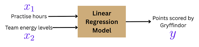
Harry wants to predict the points scored by Gryffindor in the Quidditch match tomorrow.

According to him, the score depends on two things:

• practice hours
• team energy level (rated 0–10 on match day)

Harry assumes the score (y) is some weighted combination of these two inputs (x1 and x2).

In other words, he's thinking of a linear regression model.

But here's the thing:

Harry needs to figure out the optimal weights (w₁ and w₂) so he can predict how many points Gryffindor will score tomorrow based on the practice hours and energy level.

Harry's got some data

Let's say Harry has collected data from previous matches, and it looks like this:

Now, we're assuming this data came out of some linear regression model.

If we can figure out the parameters of that model, we can figure out what the expected y is even for unseen inputs.

But nothing in life is simple

It can't be that simple. To assume in the real world that y will always be some precise linear combination of x1 and x2 would be absurd.

There's always some error involved.

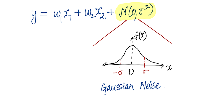
Let's say the output of the model is a linear combination of x₁ and x₂.

And let's assume this error follows a Gaussian (normal) distribution with mean 0.

That makes y a random variable!

It's centred at the linear combination (w₁x₁ + w₂x₂), but it can also deviate from it in either direction.

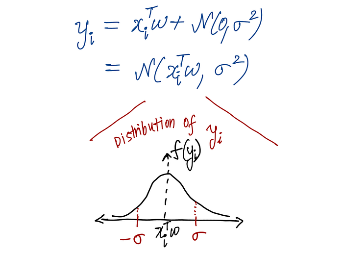
So for each datapoint i, we can write:

This probabilistic framing changes everything.

Enter the Maximum Likelihood Estimator

There's something called the Maximum Likelihood Estimator (MLE) that helps us figure out the most likely parameters given this data.

The point of it is simple:

Given the parameters w and inputs x, what is the probability (or likelihood) of obtaining these specific values of y?

How do we actually quantify this?

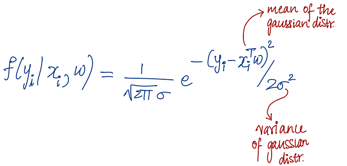
Well, remember the Gaussian distribution? It has a mathematical form that looks like this:

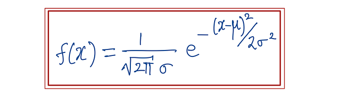
Since there's a mathematical form to it, we can figure out the probability distribution function of any specific random variable y in the data.

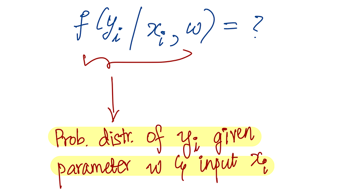
The probability that yᵢ emerged given xᵢ and w is:

This essentially tells us: how likely is it that we observed this particular value of yᵢ, given our input xᵢ and our model parameters w?

Now let's multiply them all together

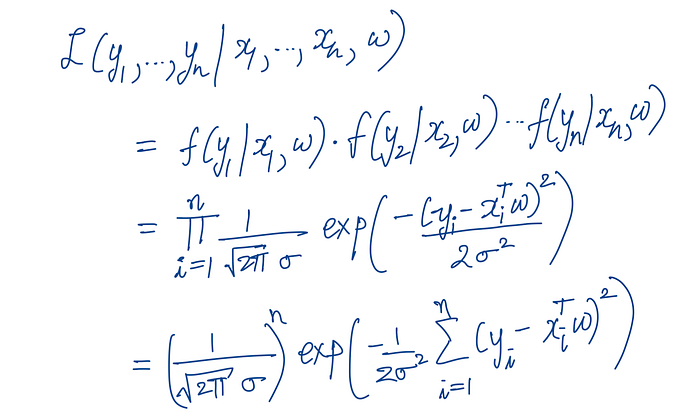
The likelihood of obtaining ALL of these yᵢ's is simply P(y₁) × P(y₂) × P(y₃) × …

We're just multiplying them together.

So the full likelihood looks like this:

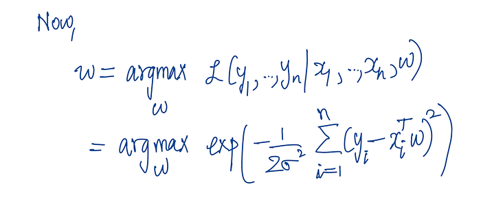
Now, if we say that the best w is the one where this likelihood is maximised, we frame it mathematically like this:

The magic happens when we simplify

To make things easier, we take the log of the likelihood (since log is a monotonic function, maximising the log-likelihood is the same as maximising the likelihood).

When we do this, the product becomes a sum, and the exponentials simplify nicely.

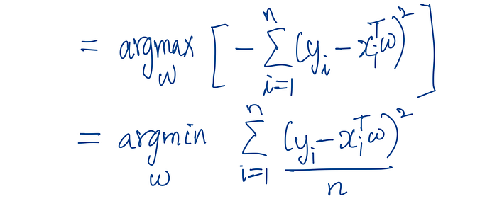
Now, maximising this log-likelihood is the same as minimising the term:

Σᵢ (yᵢ — xᵢᵀw)²

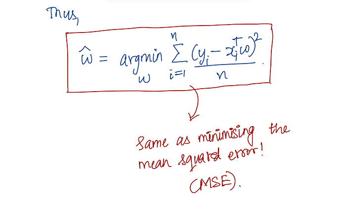
And guess what? This is exactly the Mean Squared Error (MSE) that we minimise in standard linear regression!

So essentially, the probabilistic view gives us the same MSE minimisation that we've been using all along.

What does this mean?

Here's the beautiful part:

When you minimise MSE in linear regression, you're not just arbitrarily choosing an error function.

You're actually finding the parameters that make your observed data most likely, assuming Gaussian errors.

I find this perspective way more satisfying than just saying "let's minimise error".

Thanks for reading!

If you like learning AI concepts through easy-to-understand diagrams, I've created a free resource that organises all my work in one place — feel free to check it out!

Wrapping up

In this blog, we looked at linear regression from a completely different angle: the probabilistic angle.

Every model has a probabilistic interpretation, and understanding these interpretations will undoubtedly make you a better ML practitioner, whatever kind you may be.